End-to-End Stock Market Prediction with Databricks: ETL, Model Building & Interactive Dashboard

INTRODUCTION

Building production machine learning systems for stock market prediction is less about selecting algorithms and more about designing reliable data and ML pipelines. Market data arrives late or gets corrected, feature generation must respect time boundaries, experiments need to be reproducible, and model outputs should be visible beyond notebooks. When these concerns aren’t addressed early, models become difficult to trust and even harder to operate.

This post demonstrates how to construct a comprehensive stock market prediction pipeline using Databricks. The approach emphasizes building a cohesive system rather than connecting disparate tools. The foundation relies on Delta Lake's medallion architecture for reliable data management, MLflow for structured experiment tracking and model governance, batch inference processes that generate predictions on schedule, and Databricks SQL interfaces that present results through interactive dashboards. Throughout the design, the emphasis remains on creating systems that are repeatable, observable, and sustainable as they grow.

SOLUTION ARCHITECTURE OVERVIEW

Architecture Diagram

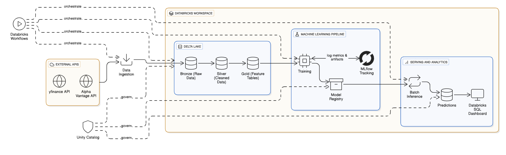
Figure 1: End-to-End Pipeline Architecture

Five components work together: Delta Lake manages data in structured layers (Bronze → Silver → Gold), MLflow tracks every model iteration, batch inference runs on schedule, SQL dashboards present findings to stakeholders, and Workflows orchestrate dependencies.

The layered approach separates concerns. Bronze captures raw market data unchanged—a complete historical record. Silver applies cleaning rules deterministically. Gold contains features explicitly designed for ML, with strict backward-looking windows preventing data leakage. This separation makes debugging straightforward and rebuilding painless when logic changes.

MLflow transforms model development from notebook exploration into managed experimentation. Every training run records parameters, metrics, and trained models. Once a configuration performs well, it's promoted to Production status—not overwritten, but explicitly versioned. Downstream jobs load "Production" by name, decoupling prediction code from training logic.

Batch inference jobs run daily, generating predictions from the current production model and appending results to Delta. Historical archives enable performance analysis: Were predictions accurate? Which features mattered most? What changed between good and bad periods?

SQL dashboards expose predictions without requiring code access. Traders see today's predictions. Leadership monitors model accuracy trends. Stakeholders understand what's happening without intermediate explanations.

Workflows coordinate execution order. If ingestion fails, features don't compute. If features are incomplete, inference doesn't run. If inference fails, dashboards don't refresh. This prevents cascading failures and ensures consistency.

DATA INGESTION AND ETL PIPELINE WITH DELTA LAKE

The ingestion layer defines the reliability boundary for the entire pipeline. In financial data systems, correctness, traceability, and reproducibility matter more than raw ingestion speed. Market data may arrive late, be revised by the source, or need to be reprocessed. This pipeline treats stock price data as a long-lived production asset rather than a transient dataset.

Bronze Layer: Immutable Raw Storage

The Bronze layer is intentionally simple: append raw market data unchanged, add only ingestion metadata (timestamp, source, batch ID), never modify anything later. This creates an auditable record and enables rebuilding downstream tables deterministically.

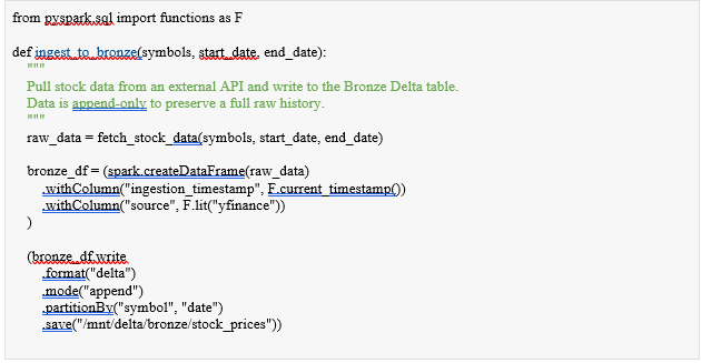
Why Delta instead of Parquet? ACID transactions prevent concurrent jobs from corrupting shared data. Schema enforcement catches upstream format changes immediately. Time-travel lets you query past table versions—critical when debugging or rerunning analysis on historical conditions.

Silver Layer: Cleaned and Normalized Data

Silver handles deduplication (keeping the most recent price correction), converts timezones consistently, filters invalid records (null prices, negative volumes), and derives basic indicators. Unlike Bronze, Silver tables can be fully recomputed when logic changes.

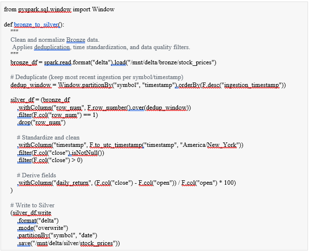
Using overwrite in the Silver layer is intentional. Since all transformations are deterministic and sourced from immutable Bronze data, the table can be safely rebuilt to incorporate logic changes, late-arriving records, or upstream corrections.

Optimize for query performance:

To keep query performance predictable as data grows, the Silver table is periodically optimized. OPTIMIZE compacts small files created during ingestion and rewrites data layout for faster reads.

ZORDER physically clusters data by timestamp. Since downstream feature jobs query specific date ranges, this dramatically accelerates queries and reduces scan costs.

Table health can be inspected using DESCRIBE DETAIL, which provides file counts and storage statistics useful for monitoring compaction effectiveness.

FEATURE ENGINEERING FOR STOCK PREDICTION

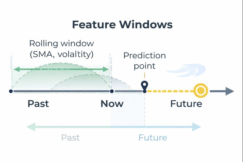
Figure 2: Feature Window

The gold layer contains the actual features used by models. Here's the critical constraint: every feature must compute from information available before the prediction date. The target variable uses a forward shift, making the prediction task explicit without ambiguity.

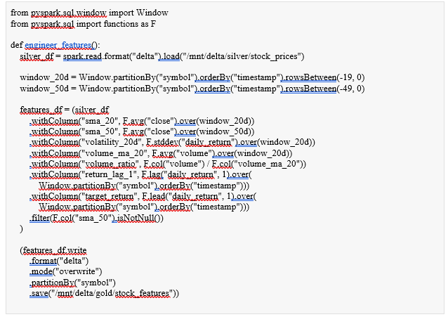
This approach prevents a subtle but critical error: using tomorrow's data to predict tomorrow. The backward-looking windows and forward-shifted target enforce correct temporal boundaries. Training respects these constraints, so inference will too.

MODEL BUILDING AND TRAINING WITH MLFLOW

With a stable and versioned feature table in place, model development becomes a controlled engineering process rather than an exploratory exercise.

Algorithm Selection

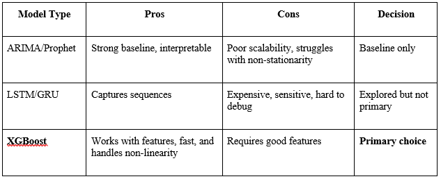
Before building anything complex, establish baselines. Classical time series models (ARIMA, Prophet) are interpretable and work with sparse data, but struggle with non-stationary behavior. Tree ensembles (XGBoost, Random Forest) leverage engineered features and handle non-linearity naturally. Deep learning (LSTM, Transformers) excels at sequences but demands large datasets and introduces operational complexity.

For daily batch forecasting, XGBoost strikes the right balance: good accuracy, fast training, straightforward feature importance, and stable in production.

Setting Up MLflow Experiments

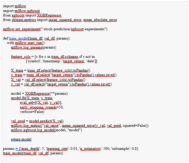
Track every training attempt systematically. MLflow records hyperparameters, validation metrics, and model artifacts for every run, making it trivial to compare approaches and understand what worked.

Comparing Multiple Models

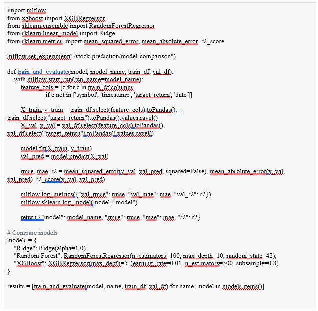
With features finalized and versioned, model training becomes a repeatable workflow rather than an ad hoc exercise. For training, features are converted to Pandas DataFrames. This keeps model APIs simple and is appropriate for moderate data volumes. When data size grows, the same pipeline can be extended to distributed training without changing how experiments are tracked or promoted.

Multiple algorithms are evaluated side by side using a shared training and validation split. Each run is logged to MLflow, capturing parameters, evaluation metrics, and the resulting model artifacts.

The comparison highlights a familiar trade-off. Linear models provide fast, stable baselines but struggle to capture non-linear market behavior. Ensemble methods improve accuracy but increase training cost. In this case, XGBoost delivers the best balance, achieving lower error metrics while remaining operationally stable for batch forecasting.

Model Comparison Results:

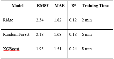
XGBoost wins on metrics while maintaining practical training time. The MLflow UI makes comparing runs trivial: filter by experiment, sort by metric, and examine details on demand.

Hyperparameter Tuning and Model Promotion

With XGBoost selected, tune hyperparameters systematically. Each variant is logged, creating a searchable history of what was tried and why something succeeded or failed.

Rather than treating trained models as notebook outputs, the best-performing run is registered as a named model in the MLflow Model Registry. This establishes a durable reference that can be used consistently across training, inference, and monitoring jobs.

The registry captures:

● The exact run that produced the model

● Associated parameters and evaluation metrics

● The model artifact itself

This step turns experimentation output into a managed asset.

Promoting the Model to Production

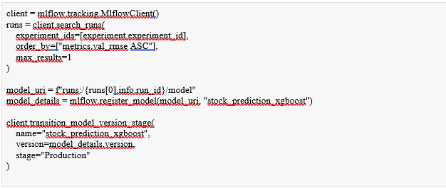
Registration alone does not make a model active. Promotion is an explicit decision.

After evaluating all runs, the model with the lowest validation error is promoted to the Production stage in the registry. This creates a clear contract: any job loading the Production model will always use the currently approved version.

This approach avoids hard-coded paths or manual artifact handling and allows model updates to be controlled and auditable.

At this point, the production model is:

● Versioned

● Traceable to data and code

● Safe to consume by downstream systems

Only after this step does inference begin.

BATCH INFERENCE

With a model explicitly marked as Production, batch inference jobs can load it by name rather than by run ID. This decouples prediction workflows from training and allows models to be updated without changing inference code.

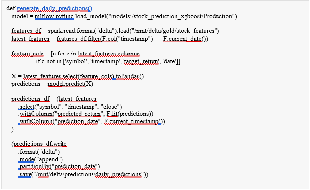
Appending rather than overwriting preserves prediction history. Later, you'll compare predicted returns against actual returns to measure accuracy and identify periods when the model struggled. This historical record informs retraining decisions and feature improvements.

Interactive Dashboard

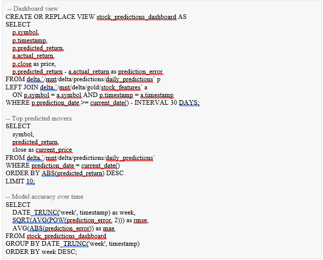
Predictions are surfaced through Databricks SQL, providing a simple, query-driven interface for reviewing model outputs. This layer is designed for analysts and business users who need visibility into results without interacting with notebooks or code.

Creating SQL Queries

We create a small set of SQL views that support common analytical questions: recent predictions, top movers, and model accuracy over time.

Building the Dashboard

Create a Databricks SQL dashboard with three visualizations:

Recent Predictions (Table): Display vw_top_movers showing top 10 predicted gainers and losers with confidence levels
Accuracy Trend (Line Chart): Plot vw_weekly_performance showing RMSE and MAE over 12 weeks to spot degradation
Error Distribution (Histogram): Show distribution of prediction errors—normal distribution is good, skewed errors suggest systematic bias

Refresh every 6 hours after market close. Share with stakeholders as read-only views—they see results without accessing data directly.

ORCHESTRATION

Databricks Workflows coordinate the end-to-end pipeline, ensuring ingestion, feature generation, and inference run in the correct order and on a predictable schedule

Creating a Workflow

● Access Workflows from the left sidebar

● Create a new job and add tasks:

○ ingest_data: runs the 01_ingest notebook.

○ clean_data: depends on ingest_data and runs 02_clean

○ Repeat for feature engineering, training (if retraining is required), and inference

● Set a schedule using a cron expression (for example, 0 0 6 * * ? for daily runs at 6 AM)

● Configure alerts to notify the team on failure.

CONCLUSION

This pipeline demonstrates how Delta Lake, MLflow, and Databricks SQL work together to create a production stock prediction system. The architecture handles data versioning, experiment tracking, and operational monitoring in a unified platform.

The system processes 50 stocks with 2 years of data in approximately 30 minutes, scales to 500+ symbols with minimal changes, and provides automated daily predictions with dashboard visibility.

In practice, production ML depends more on reliable infrastructure than on complex algorithms. This pipeline proves that with the right foundation, building and maintaining prediction systems becomes straightforward engineering rather than constant firefighting.

REFERENCES

[1] Eric Zivot, Jiahui Wang. (2006). Modeling Financial Time Series with S-PLUS. Springer.

[2] Databricks. (2022). Introducing MLflow Pipelines with MLflow 2.0. https://www.databricks.com/blog/2022/06/29/introducing-mlflow-pipelines-with-mlflow-2-0.html

[3] MLflow for ML Model Lifecycle. Databricks on AWS. (2025, June 10). https://docs.databricks.com/aws/en/mlflow/

[4] Databricks. (2024). Delta Lake: Reliable Data Foundations. https://delta.io/

[5] Databricks. (2024). MLflow: Machine Learning Lifecycle Management. https://mlflow.org/

[6] Chen, T., & Guestrin, C. (2016). XGBoost: A Scalable Tree Boosting System. In Proceedings of the 22nd KDD International Conference on Knowledge Discovery and Data Mining.

[7] MLOps Workflows on Databricks. Databricks on AWS. (2024, December 18). https://docs.databricks.com/aws/en/machine-learning/mlops/mlops-workflow

[8] Databricks. (2024). Structured Streaming: Real-Time Processing. https://docs.databricks.com/en/structured-streaming/

[9] Lakehouse Storage. Databricks. (n.d.). https://www.databricks.com/product/lakehouse-storage

[10] Armbrust, M., Ghodsi, A., Xin, R., & Zaharia, M. (2021). Lakehouse: A New Generation of Open Platforms that Unify Data Warehousing and Advanced Analytics. In Proceedings of the 2021 ACM SIGMOD International Conference on Management of Data.